Thursday 28 February 2013

Persistence in the Urban Environment : 1

Anyone reading this blog should have realised that I am interested in using maps to understand how the environment we live in has changed over time. I know I share this interest with many other OSMers. There have been many proposals, and discussions about how we might use some of the principles and technologies of OSM to create maps representing an area at some historical time point. I am greatly heartened that a new mailing list (http://lists.openstreetmap.org/listinfo/historic) has appeared for interested parties to share ideas on this subject:

Wollaton Park Estate from the E, (June 1928)


One problem which has exercised my mind, and particularly from my exercise at looking at the OSM edit history of Berlin, was how adding a history (or time) dimension to geographical data might impact on data volume. In thinking about this I have been struck that a very large proportion of the urban environment of cities in Europe and North America is remarkably static. This was brought home by the recent availability of historical aerial photographs of Great Britain (at the Britain from Above website).


Justifying the accuracy of OSM

Yesterday I came across a blog post on the OSM-GB site: this is a project hosted at Nottingham University which is about "Measuring and Improving the Quality of OpenStreetMap for Great Britain".

Although I've been aware of this project for a while it's never appeared to have much visibility within the OSM community. In part this is because it is aimed at certain classes of professional GIS users, and many of its services are WMS or WFS based. Tom Chance and James Rutter both seem to be pleased with some of the things it can do.

The blog post is concerned with 'conflating' an Ordnance Survey OpenData set (VectorMap District - VMD and OSM). VMD is the vector data underlying the StreetView tiles (roughly 1:10k scale) and the road centrelines are likely to be more accurate than OSM. It is (perhaps deliberately) lacking in some attribution (notably road names), and is designed for rendering (roads and waterways under bridges don't exist).

Only major (motorways, A- and B-roads are named and numbered). It is this latter set which has been compared with OSM in the conflation process. All differences are shown on the OSM-GB slippy map on the front page of the website. However, the conflation process assumes that the VMD data is always better than OSM. Unfortunately, one of the examples highlighted in the blog is a case where OSM is correct and the Ordnance Survey are wrong. Like a lot of mappers I do care about the accuracy of the data: I hate to get things wrong, and if I'm not sure or don't have enough information I'll try and ensure that this is shown in the tags.

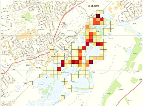
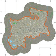
I've borrowed the image of Gregory Street, Lenton from the OSM-GB blog, which shows the length of road where OSM and OS VMD data disagree.

Mismatched OS VMD and OSM data from OSM-GB blog.

When I surveyed this in 2009 I spent quite some time trying to work out what this stretch of road was called. At the traffic lights there is a street sign "Gregory Street leading to Lenton Lane", but the next streetname plate is not to be found until just S of the canal bridge: this one has "Lenton Lane". I took this as prime facie evidence that Lenton Lane only started beyond or on the bridge (called Clayton's Bridge). I never sorted out in my own mind whether the canal bridge is on Gregory Street or Lenton Lane: the available evidence on the ground cannot be used to resolve the issue.

House numbering also confirms this: there is row of former council houses numbered from 33 to 67. If Lenton Lane started at the junction with Old Church Street then one would expect the numbering to start from 1.

Last night I did some more research to make sure I hadn't got this completely wrong. There are a good number of pieces of evidence to support my original mapping, plus one which doesn't.
  • Inspection of the Nottingham City Council GIS shows that these have a street address of Gregory Street and a postcode of NG7 2NL. House numbering is continuous from Abbey Bridge junction (the former Red Cross building is 31, to the last house next to Kirk’s auctioneers). This accords with m own mapping of the numbers for these houses. Similarly the Red Cow also has a Gregory Street address, even if the current management seem to think it's on Lenton Lane.
  • Historical mapping (for instance at Nottingham Insight) was less useful, other than to confirm that the name "Lenton Lane" is recent (it was known as Trent Lane until at least 1945). The label for "Gregory Street" always stops just before Old Church Street. However, there would have been no reason for a name change at this point, or at the crossroads: the street network was altered in the 1920s when Abbey Bridge was built as part of Jesse Boot's improvements associated with University Park.
  • The Lenton Local History Society does have a page on Gregory Street, and this shows that the Red Cow pub was on this street.
  • A Historical Street Directory, Wright's Directory of 1911, accessible on the University of Leicester website covers Gregory Street on page 70. This shows that existing locations such as the Red Cow Pub and Trevithick's Boatyard had Gregory Street addresses at that time.  
When VMD, OS locator and other products first became available we found quite a number of errors including non-existent roads, incorrectly named roads and misspelt names. In fact a tag notname was used to highlight these for feedback to the Ordnance Survey. However, disagreements about changes of names along a single highway (as in this case) would not have been picked up by this process because we were not looking for bounding box differences. See for instance Robert Scott's OS locator Musical Chairs.

I have discussed some of these issues before (for Kenyon Road). Once again I have spent some time trying to make sense of the house numbers, street signs, old maps etc.. In other words I conflated far more information than just two map sources before arriving at my decision. I know that Chris Hill has blogged about similar issues on East Yorkshire and further afield here, here and here (check Chris's blog for more). The problem which arises is that people start with the assumption that the Ordnance Survey (or any official mapping service, and these days, probably Google Maps) must be more accurate. OS data is certainly more complete, although some private roads may be missing.

I think that this means that OSM-GB need to work towards a more nuanced view of how the various aspects of completeness, and accuracy, and how that in turn determines authoritativeness. I'd also like to see outputs which are more likely to engage the OSM community, and then the goal of improving OSM quality is more likely to be achieved. ITO's (who I thought were involved in setting up OSM-GB) tools still look more convenient to me than WxS services.

In the ideal world OSM data would be sourced entirely separately from Ordnance Survey and equivalent mapping agencies so that their datasets could be used to cross-check each other. However, life's too short, so a lot of OSM data comes from the OS anyway. That does not mean that we should not continually check and refine the data so that more and more of it is underpinned by actual surveys and, if necessary research and local knowledge to resolve tricky problems like this. Ultimately, OSM has to build a reputation for authoritativeness, and national mapping agencies have a bit of a head start on us. Such a reputation is far more useful than any amount of metadata, or detailed explanations such as this one (which take too long to write, and read, anyway).

One could envisage some kind of multi-media experience accessed by clicking on a single OSM way which would report who had added traces, relevant photos, old maps, dictaphone and video mapping logs, old street directories etc. Many of the bits exist (traces, tagged photos on Flickr, openstreetview, ...), but not in such a way as to overwhelm the senses of someone wanting to know why they should believe in OSM!

Sunday 17 February 2013

Quicker mapping of Street Trees

OpenStreetMap with Observado tree observations KML
I have always been cautious about mapping trees on OSM - not because I don't want to, but because it is time-consuming and difficult to achieve consistency in mapping over reasonable areas. During 2008-9 (before I did OSM) I mapped about 100 Oak, Quercus robur, trees at Attenborough Nature Reserve. This took 5 separate visits lasting on average about an hour and a half. Of course I was doing other things as well, but each tree took about 5 minutes (I was also measuring the circumference (more properly Breast Height Girth). I still find this data set very useful (see below), but I did learn how time consuming the process can be.

Friday 15 February 2013

Mundane Cartography : mapping Vice Counties

VC13 West Suffolk
West Sussex (VC13) mapped using OS OpenData (Meridian2)
database right, Ordnance Survey, 2012
Late last year I grew increasing frustrated with the maps I use within MapMate for biological recording. Maps have two purposes: firstly they help in putting records in the right place; secondly, they provide a context for displaying cumulative sets of records (usually in a distribution atlas).

MapMate allows the creation of maps through an absolutely horrible interface. The vector sets which come with the product are too inaccurate for serious work. Long ago I moved to using geolocated images as an informational underlay within the product. I've used various techniques: grabs of OS Maps from the OS website, OSM maps generated with Kosmos or Maperitive, OS OpenData Tiles (StreetView, 250k etc). None has been wholly satisfactory: either they have too little information or too much. After several years of doing this I think I now have a much better idea of what is needed.

Typical recording focuses on small discrete areas: perhaps from 1 to 250 hectares in size. In these areas the ideal is to note precise positions of things like plants, insects and fungi, but location to within 100 metres is a reasonable compromise: the 6-figure grid reference beloved by British Naturalists. However, with one of my datasets containing well over 1000 records I noticed that using manual methods (looking at a map & assigning the record to a square) I was frequently 100 metres out. This was most noticeable with a Buckthorn growing on North Path at Attenborough Nature Reserve. There are a number of insects and fungi which are associated with this plant which I have recorded on this isolated tree. Over time I'd managed to place records in three adjacent 100m squares. Although I'm trying to move to direct data capture in the field this is still not possible in lots of circumstances. Therefore being able to create maps which have more pertinent information can help accurate recording a lot.

Plant Gall recording at Attenborough, record counts
OS OpenData StreetView used for recording at 100m square level

On a smaller scale the same thing happens too. For recording at the vice county level (perhaps typically 2500 km2) the currently favoured unit is the grid kilometer square or the tetrad. Again it's easy to be out by one if the map used for data entry does not have the right level of detail. I therefore wanted to create maps which I could use as a reference layer in the recording software and which had large number of visual cues to enable rapid and accurate selection of the correct grid square for recording. Obvious information includes major water bodies (lakes and rivers), larger areas of woodlands, and settlements. The road and railway network also provide useful queues. It's probably not necessary to make use of all of these, but I was interested if I could produce a simple cartographic product which could then be altered for a variety of purposes.

Long ago Richard Fairhurst had remarked that he favoured one of the OS OpenData sets, Meridian 2 or Strategi, I can't recall which, as a good base for cartography at medium scales. I'd neglected to follow this up, but recalled his argument when I started doing this. Therefore my starting point was the Meridian 2 dataset, Vice County boundaries (mean low-water line version) from NBN Gateway, and a couple of datasets showing protected areas (SSSIs and Local Nature Reserves) from Natural England.

As I wanted something fairly quick and dirty I chose Quantum GIS to do the cartography.

Firstly, I created a shapefile with the relevant vice county I was interested in, and then buffered this by 5 km to create a 'halo' to provide additional context for the map. Later I decided that I wanted to mute areas outside the county, so I created another shapefile which was the difference between the two. I achieved my goal by placing this at the top of the list of layers and making it 50% transparent.

The Meridian layers I used were, lowest layers first: Woods, Rivers, Lakes, Minor Roads, B-Roads, A-Roads, Railways, Motorways and Settlements. I added SSSI and LNR layers as hatched overlays. This produced a map which was pretty satisfactory, even though it reflects a very simple application of the Painter's Algorithm. The image below shows the QGIS workspace:

Layers showing application of Painter's Algorithm in QGIS
I've run into a few problems:
  • A number of the original vice county polygons were incorrectly formed. Although it's not too difficult to identify the problem they are quite difficult to repair. Fortunately most of these are in the far north of Scotland, so don't worry me at the moment.
  • OS Open Data provides the coast line as a polyline. I need land areas as polygons for various manipulations. I have therefore started creating land tiles corresponding to Ordnance Survey 100km grid squares. I am using PostGIS to do this.
  • Vice County boundaries reflect mean low water tides. For areas of mud flats and sand these can be a long way from the high water line (coastline). These areas need to be split out as a distinct layer below the sea.
  • Boundaries need to be changed to polylines because I don't want to show boundaries on the coast. Where two vice counties are separated by a sea channel some further work needs to be done.
I'd also like to add some more data:
  • Shaded Relief
  • Contours or Hypsometric tints
  • Urban area landcover
  • Boundaries of National Parks & Areas of Outstanding Natural Beauty (AONB)
  • Parkland 
  • Settlement names for larger settlements and different symbols for settlements by size.
VC49, anachronistically still called Caernarvonshire, has been my test area for some of these changes.

VC49 Caernarvonshire (experimental)
VC49 Caernarvonshire with hill-shading and hypsometric tints. Note coastline issues.
Now that I have the basic idea I've got the core of the data in PostGIS. There is plenty of scope for modifying the cartography for different purposes. In particular a muted or greyscale style is desirable as an orientation layer for thematic maps. I've only just started playing with these (see below)

VC21 Middlesex (experimental muted colours, grey on pale)
VC21 Middlesex Grey on Pale
VC21 Middlesex (experimental muted colours, white on grey)
VC21 Middlesex, White on Grey

I've called this mundane cartography because there is absolutely nothing special in what I have done. I've mainly used a single dataset as is, a very simple minded version of the Painter's Algorithm, and a fairly straightforward GIS toolset.

One of the interesting things about mapping at this scale: roughly between 1:150k to 1:400k, is that there is very little data directly related to the natural landscape which it makes sense to show. Woodland, Lakes and Rivers just about covers all the areas which are likely to be useful at these scales. Natural England have a large number of datasets of special vegetation types, but many of these are barely visible even at 1:25k scales. This is particularly true now that many of these vegetation classes are much diminished in total area compared with even 50 years ago.

The reasons for not using OpenStreetMap data are very similar to those adumbrated by Richard Fairhurst: consistency, generalisation, and completeness. Mapping of woodland and water is essential for my goal: these are likely to be areas with an higher level of recording than other areas. Many large forestry areas have not been mapped, particularly in Scotland and Wales. Similarly it would have been time-consuming to try and generalise OSM data which, in the main, are too detailed for this purpose.